Integrating Inventory Into Air vs. Ocean: International transportation modal choice strategies

As firms deploy their inventories across multiple continents to serve growing markets, the costs of transportation and the direct impact of transportation modal decisions on a firm’s inventory investment requirements require careful analysis. To avoid the trap of focusing strictly on freight costs, firms must employ a transportation mode choice decision-making methodology that recognizes all the costs associated with transportation decisions. In this article, we present a modal choice decision-making methodology that combines annual cost and long-run inventory investment perspectives to identify the best transport mode choice. Additionally, we provide an analytic approach for evaluating situations where a mixed-mode transport strategy (i.e., a combined ocean and air strategy) may represent the best alternative.

We begin by reviewing a methodology first developed to determine if a Fortune 100 company should use air or ocean freight to transport finished goods between its plants and distribution centers. The firm’s manufacturing and distribution groups were at odds because manufacturing argued that an ocean strategy would require a tremendous investment in inventory that was economically unjustified, while distribution countered that the freight savings from using cheaper ocean transport outweighed the higher inventory investment costs that the ocean option would require. It turned out that each group was both right and wrong—ocean freight was more cost-efficient for certain product lines and air freight for others.

The first half of this article details our air vs. ocean methodology and illustrates the analytic results it generates. The second half introduces an enhancement to the methodology that allows planners to evaluate a mixed ocean and air inventory replenishment strategy. Through examples, we describe what situations may warrant consideration of a combined ocean/air strategy for an individual product.

The air-ocean methodology

To illustrate our methodology, we pose a hypothetical scenario in which a firm must evaluate whether to ship product by air or by ocean between two of its facilities located on different continents. Our example assumes that a firm manufactures finished goods inventory (FGI) in a plant in the Far East and distributes these products to customers in Europe from its distribution center located in Europe. We further assume that the firm supplies make-to-stock products on demand to its customers from this distribution center. Thus, it must maintain inventory at the distribution center to fill orders immediately as customers place them, and it must maintain a safety stock inventory to cover the variability in demand over inventory replenishment lead time and the variability of replenishment lead time.

Key costs to evaluate. To evaluate whether to establish air or ocean inventory pipelines to transport the firm’s products between its plant and distribution center, we must consider five major cost factors that will differ depending upon which transportation mode the firm selects. These are:

1. the freight costs;
2. the inventory carrying costs of inventory in the pipeline;
3. the inventory carrying costs of cycle stock at the receiving distribution center;
4. the inventory carrying costs of the required safety stock at the receiving distribution center; and
5. the investment cost required to produce the inventory to fill the pipeline (i.e., the average total inventory required in transit and at the distribution center).

The first four cost factors are annual recurring costs, while the fifth cost represents a one-time cost required to initiate the pipeline.

Integrating inventory investment analysis and annual costing

The annual costs can be analyzed using spreadsheet calculations once the proper supporting data have been developed (see Table 1). However, calculating the initial inventory investment and determining the return on investment associated with an inventory pipeline modal choice is not as straightforward. Investment decisions typically involve weighing an expected return against the investment necessary to generate that return. In other words, to evaluate the pipeline modal choice from a long-term investment perspective, a company must quantify both the investment and the expected return associated with each mode.

The best way to do this is to focus on incremental costs and investment. This approach views the annual incremental savings or cost avoidance associated with ocean transport as the incremental stream of income resulting from the incremental investment in an ocean pipeline. An ocean pipeline requires a larger initial inventory investment than an air pipeline because the transit time—and hence days of inventory—is longer. With the incremental annual stream of income and the incremental pipeline investment defined, one can calculate measures such as return on investment and the investment payback period. [For a discussion of additional incremental air vs. ocean considerations (e.g., inventory salvage and warehouse storage space costs), see Miller and Liberatore (2021)].

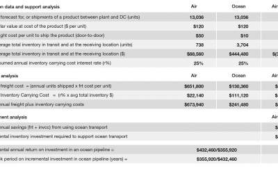
Illustrative examples. Table 1 illustrates both the annual cost and the investment analysis of our hypothetical scenario. The “annual analysis” section indicates that utilizing an ocean pipeline to transport the firm’s product from its plant to its distribution center will save $432,460 per year. The higher annual inventory carrying costs ($88,980) are outweighed by the substantially higher freight savings ($521,440) yielded by ocean.

The “investment analysis” section of Table 1 evaluates the ocean vs. air decision from two perspectives: (1) return on investment, and (2) the payback period of the investment. Dividing the annual savings ($432,460) from using ocean by the incremental inventory investment ($355,920) required to support ocean produces a 121.5% return on the incremental inventory investment. To project the number of years it will take for the additional inventory investment required by ocean to “pay for itself,” we divide the incremental inventory investment ($355,920) by the annual “ocean” savings ($432,460). This shows that in just under one year (0.8), the savings will pay for the incremental inventory investment. (As described in Miller and Liberatore, this methodology can also incorporate factors such as inventory salvage value, net present value, and others.)

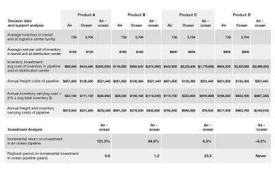
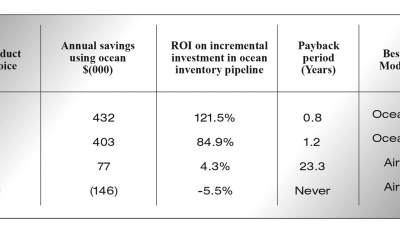
To illustrate this methodology further, consider Table 2 which summarizes an annual cost and investment analysis for four products. Product A (which has a unit cost of $120) is the same product evaluated in Table 1 while products B ($160 unit cost), C ($600 unit cost), and D ($900 unit cost) are more expensive products our fictitious firm produces and ships to its distribution center to serve European demand. The results for the four products in Table 2 suggest the best mode choice to replenish inventory from the firm’s plant to its distribution center, as shown in Figure 1.

The analysis shows that the ocean option represents the cost minimizing alternative for products A, B, and C, while for product D, air minimizes annual costs.

Importantly however, from an incremental inventory investment perspective, while the savings for products A and B from an ocean pipeline produce robust returns (121.5% and 84.9%), the ocean pipeline cost savings for product C generates only a 4.3% annual return. Further, it would require 23 years for an ocean pipeline of product C to pay for itself. Thus, the investment analysis strongly suggests that the annual savings generated by an ocean pipeline for product C would not justify the required extra inventory investment. A firm that only considers the annual freight and inventory carrying costs of transport mode alternatives, and which neglects the investment component of this decision, is vulnerable to making poor transport mode choices (e.g., selecting ocean transport for product C). Finally, the firm should clearly ship product D via air because even from an annual cost perspective, this represents the cost-minimizing choice. The high cost to carry inventory of product D resulting from its high unit cost drives this outcome.

Broadly speaking, for any product where either ocean or air transport is feasible (i.e., there are no environmental, hazardous material, safety or other product specific factors that dictate the required transport mode choice, regardless of costs ), an analysis of the annual costs and the incremental inventory investment return will produce three categories of results:

1. clearly ship by ocean;
2. clearly ship by air; or
3. ambiguous—ocean has substantially lower costs, however, the incremental inventory investment to support ocean is substantial.

For firms that have products that fall into category 3, where the annual ocean freight savings are attractive, but the required incremental inventory investment is concerning; we next review an analytic approach that offers additional perspective. Specifically, we illustrate a methodology to evaluate a “combined and planned” ocean and air inventory replenishment pipeline strategy.

Background on analytic approach

The following approach evaluates the potential value of using a joint ocean/air replenishment strategy. It is important to note that a firm’s practical ability to employ this combined strategy may be limited to specific replenishment situations, and we will discuss this point later. To illustrate our analytic approach, we consider Product B from Table 2, and assume that our firm has a corporate financial policy (as some firms do) stipulating that $400,000 is the maximum level of inventory investment allowed for any single product. While the all-ocean option for product B would save $402,800 annually, has an incremental inventory investment return of 84.9%, and a payback period of just 1.2 years, it would require an inventory investment of $592,640 to facilitate an ocean pipeline. Therefore, employing an all-ocean strategy for Product B would necessitate an inventory investment level that exceeds the maximum corporate limit.

However, given the potential significant costs savings of shipping Product B by ocean, we want to explore the following questions.

1. Could our firm limit its inventory investment in Product B to $400,000, and by supplementing regularly planned ocean shipments with “additional” emergency air shipments as needed, still generate substantial annual savings compared to an all-air replenishment strategy? 
2. Further, would this approach yield an acceptable return on investment?
3. Finally, could this be done without materially degrading the DC’s fill rate to its customers?

The following describes the basic steps we take to evaluate the potential efficacy of a planned ocean/emergency air strategy. We begin with a brief illustrative scenario, and then detail the analytics.

The following steps summarize the analysis to evaluate this potential ocean/emergency air scenario.

1. Determine the projected annual lost sales units, lost profits, and lost revenues for the all-air replenishment strategy. (i.e., What would the lost sales units, profits and revenues be if the DC provided an annual fill rate of 98% outbound to its customers).
2. Determine the projected annual lost sales units, profits, and revenues that an all-ocean replenishment strategy would create if total inventory investment was constrained to the maximum corporate level allowed: $400,000 for Product B. (i.e., no emergency air shipments are allowed.)
3. Determine the projected total annual costs of a combined ocean/emergency air shipment strategy designed to maintain (or come close to) the same planned fill rate target (i.e., 98%) that an all-air strategy would generate.
4. Evaluate whether the planned target fill rate (or an acceptable fill rate close to the target) can be produced by a combination of regular ocean shipments supplemented by emergency air shipments as required.

To complete step 1 through step 4, one can develop a Monte Carlo simulation model, or more simply utilize several Excel functions in a spreadsheet analysis. Briefly, the Excel functions include using a random number generator to project variable daily demand, and employing another Excel function that calculates the probability values associated with a normal distribution of demand. We developed both a Monte Carlo simulation model (contact the authors for more information on the Monte Carlo simulation model) and a simpler Excel spreadsheet to evaluate our illustrative scenario. Tables 3, 4, 5, and 6 present results based on the spreadsheet approach.

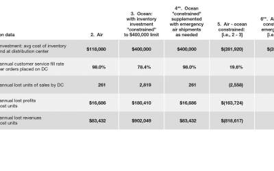
Table 3 compares the DC customer service fill rates as well as the lost sales units, profits and revenues projected under three scenarios.

1. The plant replenishes inventory at the DC only by air (column 2).
2. The plant utilizes only ocean shipments to supply the DC (column 3) and the inventory investment in Product B is constrained to $400,000.
3. The plant employs both ocean and emergency air shipments to supply the DC (column 4).

Table 3 shows that an all-air strategy will facilitate a 98% fill rate by the DC, while an all-ocean strategy generates only a 78.4% fill rate with inventory investment constrained to $400,000. (Recall from Table 2 that Product B would require an inventory investment of $592,640 for the all-ocean strategy to match the fill rate of the air strategy.) As shown in column 4, initially we assumed that by using an “inventory constrained” ocean strategy supplemented by emergency air replenishment shipments, the DC would provide the identical fill rate (98%) as would the all-air strategy. We relax this assumption later in Tables 5 and 6.

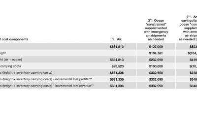
Table 4 contrasts the annual costs of the all-air replenishment strategy to those of the inventory-constrained ocean/emergency air approach. Recall that emergency air shipments would occur as needed throughout the year whenever the analysis performed by inventory planners at the beginning of each inventory review period (e.g., once per week) indicates that the DC’s inventory level for that review period is or will drop below the minimum target level. Column 3 displays the emergency air and ocean freight annual expenses to ship Product B from the plant to the DC for this inventory constrained ocean/emergency air scenario. Column 4 shows that the combined ocean/emergency air replenishment plan would save just over $348,000 per year. This annual savings is lower than that of the all-ocean strategy shown in Table 2 ($402,800) where the inventory investment ($592,640) is determined by the inventory level required to generate a 98% fill rate rather than by a corporate limit of $400,000. Also note in Table 4 that there are no incremental lost profits or revenues associated with the combined ocean/emergency air strategy, as it is assumed that the emergency air shipments allow the DC to provide a 98% fill rate to its customers, just as an all-air strategy would.

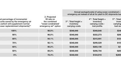
Table 5 offers sensitivity analysis results for the ocean/emergency air scenario. In practice, it may not be possible to assure that an ocean/emergency air replenishment strategy will facilitate an equal customer service fill rate by the DC to its customers as would an all-air replenishment strategy. Thus, Table 5 addresses both the service and cost implications of utilizing an ocean/emergency air approach.

To clarify the correct interpretation of the results in Table 5, we make the following definition: Incremental lost sales units = (sales units lost under an all-air strategy) – (sales units lost in an inventory-constrained all-ocean strategy). For this example, column 5 in row 3 of Table 3 shows incremental lost sales units = 2,558.

Briefly, the sensitivity results presented in Table 5 are as follows:

• Column 1 displays the assumed percentage of incremental “lost sales” units that would be saved by the emergency air shipments. Thus, in column 1, 100% indicates there will be no incremental lost sales in an ocean/emergency air strategy (i.e., the emergency air shipments prevent any incremental lost sales); 90% indicates all but 10% of the incremental lost sales units are saved; 0% means that emergency air shipments do not save any incremental lost sales.
• Column 2 shows the resulting decline in fill rate the DC would provide customers as the percentage of incremental lost sales saved by emergency air shipments declines.
• Columns 4 and 5 calculate the resulting decrease in the annual cost savings generated by the ocean/emergency air strategy as the percentage of lost sales saved by emergency air shipments drops.
• In column 4, the lost profits are subtracted from the projected annual total cost savings of an ocean/ emergency air plan. For example, if emergency air shipments save only 90% of the  otential incremental lost units, then the lost profits from the 10% of incremental lost units not prevented reduce the annual savings from $348,646 to $332,273 (row 2).
• Similarly in column 5, the lost revenues are subtracted from the cost savings of an ocean/emergency air strategy [e.g., as shown in row 2, if emergency air shipments save 90% of the incremental sales units potentially lost, the lost revenues reduce the annual savings to $266,784 from $348,646].

The following discussion illustrates how a firm could employ the results in Table 5 to decide if an ocean/emergency air strategy warrants further consideration. First, we focus on the cost results. Row 1 shows that for Product B, if the ocean/emergency air approach can prevent any incremental lost sales (100%) and deliver the identical fill rate (98%) as an all-air approach, this combined transportation mode strategy would save just more than $348,000 per year as previously shown in Table 4.

However, in rows 2 (90%) through 7 (0%), we evaluate the impact of the potential lost profits and lost revenues. These rows show that if the emergency air shipments do not prevent losing some or all of the potential incremental lost sales units, the annual savings of the ocean/air strategy diminish significantly, and when lost revenues are considered become actual losses for the firm if 50% or more of the potential incremental lost sales are lost. Thus, Table 5 illuminates the potential benefits (cost savings) and risks (increased costs) of the combined ocean/air strategy. Next, Table 6 enhances this cost analysis utilizing the “investment” methodology.

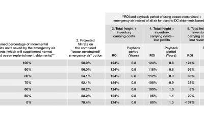
Table 6 demonstrates the contrasting perspectives portrayed of an ocean/air strategy depending upon whether one considers just annual freight and inventory carrying costs, or if one also includes potential lost profits and revenues. Column 3, which evaluates annual freight and inventory carrying costs, indicates that the combined ocean/air strategy would generate a high ROI (124%) and a rapid payback (0.8 years) on the incremental inventory investment. Because this column does not consider the impact of lost profits or revenues, the ROI and payback period values remain constant in rows 2 (90%) through 7 (0%)—i.e., the scenarios where there are lost profits and revenues. However, we cannot assume that an ocean/air strategy will result in no incremental lost sales. This assumption may not be correct and may be difficult to evaluate accurately before the implementation of this strategy.

Thus, columns 4 and 5 of Table 6 evaluate the potential reality that may materialize by including potential lost profits and lost revenues in the analysis. For Product B, one observes that if the emergency air shipments prevent only 50% of the potential lost sales units from being lost (row 6), while the ROI and payback including the costs of lost profits (column 4) are still quite good (95% and 1.1 years), adding potential lost revenues to the analysis indicates that the ROI turns negative, and the incremental inventory investment is never paid off. On the other hand, if emergency air shipments can save 80% (row 3) or more of the incremental lost sales units, then the ocean/air strategy may warrant further consideration—even after including lost revenues.

Individual firms will weigh the relative importance of lost profits and lost revenues in their analyses differently. Briefly, we simply note that Tables 5 and 6 provide an enhanced perspective to evaluate the potential cost savings, if any, of an ocean/air strategy. Further, in the case of ocean/air strategies, relying strictly on analyses based only on annual freight and inventory carrying costs is insufficient, and evaluating the potential impact of incremental lost profits and revenues is critical.
We now consider other factors that will influence the potential benefits and practicality of this combined strategy.

Non-cost factors to consider in evaluating a combined ocean/air strategy

Supply chain decisions invariably require consideration of both costs and other factors such as customer service implications and risk levels.

To illuminate these non-costs when accommodating a joint ocean/air strategy, we offer an illustrative list of general considerations to evaluate.

An example of a network well-positioned to accommodate a combined strategy.

The following represents the type of network that would have a high probability of successfully implementing a joint ocean/air strategy for individual products.

1. A firm has a plant that produces many products that it ships to the firm’s DC and maintains make-to-stock inventories of each product to serve its (the DC’s) customers.
2. The plant makes regularly scheduled (e.g., weekly) replenishment shipments of these products to the receiving DC.
3. The plant utilizes both air and ocean to ship containers with inventory replenishments to the DC. High-value products are shipped by air and lower-value products move by ocean.
4. The plant has air and ocean freight carriers with whom it has well established relationships and/or contracts for its regularly scheduled shipments.

The network just described represents the perfect situation for a firm to implement an ocean/emergency air strategy to replenish the inventory of any products at the DC for which this approach could generate significant cost savings. To illustrate, assume the plant regularly produces a broad mix of: (1) inexpensive products, (2) expensive items, and (3) products that are mid-range in cost. On a network such as this, a firm could readily prototype and then fully implement an ocean/emergency air strategy for a selected subset of its products.

Specifically, each week (or replenishment planning cycle) for those products supported by ocean/air replenishment, planners determine if emergency air shipments of each product are required, or if regular ocean replenishment is sufficient. Then the appropriate inventory quantities of a product could be loaded into ocean and/or air containers. The key point is that because the plant regularly loads both ocean and air containers each week, utilizing a combined ocean/air strategy for selected products adds minimal, if any, operational complexity. It simply requires loading the correct number of pallets of a product into the correct container type (i.e., air or ocean), and then loading the containers on the correct vehicle. Therefore, in this network, a combined ocean/air strategy represents a very feasible option operationally.

Illustrative general considerations to evaluate. The following list, while not comprehensive, illustrates the types of factors that a firm must consider before implementing a joint ocean/air strategy for an individual product.

1. Is this a practical strategy that can be implemented with minimal risk?
2. Does the firm have a significant number of products that are candidates for joint ocean/air replenishment?
3. Are the potential cost savings significant enough to justify the risks?
4. Does the firm have products that are good candidates to pilot an ocean/air strategy?
5. What is the feasibility of switching back to an all-air strategy if service issues arise?
6. If the firm currently uses an all-air strategy, does it have sufficient storage space at its receiving DC to house the higher inventory levels required by an ocean/air strategy?
7. Does the firm have strong relationships/contracts with ocean and air carriers that allow it to flex volume between ocean and air as needed; and do its carriers consistently have capacity available to accommodate varying flow levels?

Summary

We began this article by presenting a methodology to evaluate quantitatively the ocean vs. air transport mode inventory pipeline replenishment decision. A key feature of this methodology includes integrating inventory costs into the transport decision. We then introduced an enhancement to this binary choice methodology (i.e., air or ocean) by illustrating how a combined ocean/air replenishment strategy can be assessed. This enhanced methodology facilitates a quantitative evaluation of situations where the annual cost savings of an ocean replenishment pipeline are substantial, however, the inventory investment required to facilitate these annual savings may exceed levels a firm is comfortable undertaking.

A key takeaway from these methodologies is that the return on the incremental inventory investment required to support an ocean (or ocean/air) pipeline, as well as annual costs (i.e., freight and inventory carrying costs) must both be considered in choosing between an air, ocean, or combined ocean/air replenishment strategy. Further, in the case of the ocean/air option, it is critical that a firm factor the impact of potential lost sales into its analysis.

Finally, we note that these methodologies can be expanded to include other factors typically found in investment analyses (e.g., pipeline salvage value, net present value analysis, etc.). •

Editor’s note: Small portions of this article previously appeared or were adapted from Miller (2016).